Bearded-android-docs

Created Thursday 21 November 2013

• http://page.mi.fu-berlin.de/rojas/neural/chapter/K7.pdf
• http://jeremykun.com/2012/12/09/neural-networks-and-backpropagation/

Motivation for the Backpropagation Algorithm

• Goal: for fixed training example `bb x`, we want the NN to output a specific output `bb t`.
• We need to somehow modify the weights `bb w` so that the output is as close as possible to `bb t`.
• We can measure the difference between the actual output and expected output and somehow minimize the error.
• The total error measures the difference between the actual and expected outputs.
• The total error is actually function of the weights! (Each training example is fixed. The weights are the only parameters that can minimize the error function.)
• The total error is continuous and differentiable! (Each impulse function is continuous and differentiable. E is built via composition and summation of the impulse functions. Thus, its gradient exists.)
• As a result, we can use the method of gradient descent to minimize the error function and find the values of the weights. In a nutshell, this is the backpropagation algorithm.

Derivation of the Backpropagation Algorithm (Sort of)

The Gradient of the total error `E`

Consider a single-layer network with only a single neuron `(bb w,phi)` and a single training example `(bb x, bb t)`. Since the NN has a single neuron, `bb t` is a one-dimensional vector i.e., `bb t=t`, a scalar.

Then the total error is `E=E[1]`.

But wait there's more! Since the NN has only a single neuron, the output is just the value of the neuron's impulse function `f`, so

`\ E = 1/2 ||f(bb x) - t||^2 = 1/2 ||phi(bb w * bb x) - t||^2 = (phi(bb w * bb x) - t)^2`

where E is a function of `bb w`.

The gradient of E is

`\ grad E = ((dE)/(dw_0),... ,(dE)/(dw_k))`.

Let's compute a `(dE)/(dw_j)`.

`\ (dE)/(dw_j) = (d)/(dw_j) [phi(sum_k w_k x_k) - t]^2`

`t` and each `x_k` are constants. Also, each `w_i != w_j` is constant. So the expression is really of the form

`\ (dE)/(dw_j) = (d)/(dw_j) (phi(C + w_j x_j) - D)^2`

where `C` and `D` are constants. Applying the chain rule twice (once on the squared term and then on `phi`)

`\ \ \ (dE)/(dw_j)`
`\ \ = 2(phi(C + w_j x_j) - D) xx (d)/(dw_j)(phi(C + w_j x_j) - D)`
`\ \ = 2(phi(C + w_j x_j) - D) xx phi'(C + w_j x_j) xx x_j`
`\ \ = 2[phi(sum_k w_k x_k) - t] xx phi'(sum_k w_k x_k) xx x_j`

Phew! Let's make a simplification. `phi(sum_k w_k x_k)` is just the output `o` of the neuron, so

`\ \ (dE)/(dw_j) = 2(o - t) phi'(o) x_j`

The Backpropagation Algorithm

The gradient points in the direction of steepest ascent, so if we want to go to the minimum, just travel backwards along the gradient. In other words, add a negative multiple of `(dE)/(dw_j)` to the current weight `w_j` to go towards the minimum of `E`:

`\ \ w_j = w_j - eta (o - t) phi'(o) x_j`

(We drop the "2" since it gets absorbed by `eta`. `eta` is called the learning parameter.)

Let's step back for a minute. We're adjusting the weights (which are the real inputs) so that the error function E is at its global minimum (hopefully). The problem is how can we be sure its a global minimum? how can we be sure the adjustment doesn't overshoot the minimum? how can we be sure we don't oscillate near the minimum?

Enter the momentum.

`\ \ w_j = w_j - eta (o - t) phi'(o) x_j + alpha w_j[prev]`

where `alpha` is the momentum parameter and `w_j[prev]` is the value of `w_j` from the previous iteration of the backpropagation algorithm.

The backpropagation algorithm repeats this process until the error E is smaller than a preset value.

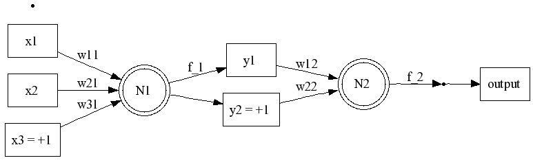
More generally, we can apply the same reasoning to an NN with more than one neuron and more than one layer. In the general case, the formula for a gradient is a function of the gradients in the next layer. Hence, the name backprogapation since you must start in the output layer and work backwards to find the weights.

Backlinks:

Attachments: